When designing high-speed analog circuits, op-amp stability is a paramount concern. An unstable amplifier will oscillate, injecting unwanted high-frequency noise into your signals or rendering the output entirely useless. This technical note outlines the fundamental physics of feedback-induced oscillations, how to evaluate phase margins, and practical ways to design compensation networks.
The Feedback Loop and Instability
Any operational amplifier circuit employs negative feedback to establish a predictable closed-loop gain. The gain block is defined by the open-loop gain $A(s)$ and the feedback factor $\beta$. The overall closed-loop transfer function is given by the classic equation:
\[A_{CL}(s) = \frac{A(s)}{1 + A(s)\beta}\]If the quantity $A(s)\beta$ (the loop gain) approaches $-1$ at any frequency, the denominator becomes zero, resulting in infinite gain and sustained oscillations. In physical terms, this occurs when:
-
The magnitude of the loop gain $ A(s)\beta = 1$ (0 dB crossover frequency, $f_c$). - The phase shift around the feedback loop reaches $-180^\circ$.
Calculating and Measuring Phase Margin
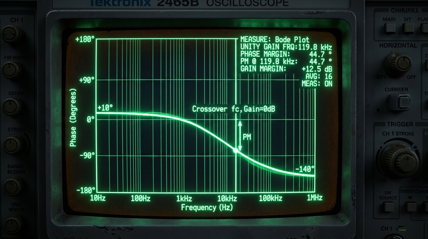
Phase margin (PM) is a metric that measures how far an amplifier is from instability. It is defined as the difference between the loop gain phase and $-180^\circ$ at the crossover frequency $f_c$ where the loop gain is exactly
\[$0 \text{dB}$ ($|A(f_c)\beta| = 1$): \text{PM} = \angle A(f_c)\beta + 180^\circ\]- PM > 60°: Excellent stability. The system has minimal overshoot and ringing in response to step inputs.
- PM = 45°: Marginally stable. Expect some overshoot and ringing, but the signal will eventually settle.
- PM < 30°: Highly unstable. The circuit is prone to sustained oscillations with temperature or load changes.
To measure this on the workbench, we sweep the frequency and plot the magnitude and phase, identifying the crossover point on a Bode plot:
Python Simulation of Phase Margin
We can model the open-loop response of a dual-pole op-amp and calculate its phase margin using a simple Python script:
1
2
3
4
5
6
7
8
9
10
11
12
13
14
15
16
17
18
19
20
21
22
23
24
import numpy as np

def calculate_phase_margin(f_crossover, poles):
    """
    Calculates phase shift and margin at crossover frequency.
    poles: list of pole frequencies in Hz
    """
    phase_shift = 0.0
    for pole in poles:
        # Each pole introduces phase lag: -arctan(f/fp)
        phase_shift -= np.arctan(f_crossover / pole)

    # Convert from radians to degrees
    phase_deg = np.degrees(phase_shift)
    phase_margin = 180.0 + phase_deg
    return phase_deg, phase_margin

# Define poles of a generic dual-pole amplifier
opamp_poles = [100.0, 15000.0]  # Pole 1 at 100 Hz, Pole 2 at 15 kHz
fc = 12000.0                    # Crossover frequency in Hz

phase, margin = calculate_phase_margin(fc, opamp_poles)
print(f"Phase Shift at {fc/1000:.1f} kHz: {phase:.1f}°")
print(f"Calculated Phase Margin: {margin:.1f}°")
Practical Compensation Techniques
If your simulation or measurements indicate a poor phase margin (less than 45°), you can implement several compensation techniques:
- Dominant-Pole Compensation: Artificially adding a low-frequency pole to roll off the gain before the high-frequency phase shifts reach critical levels.
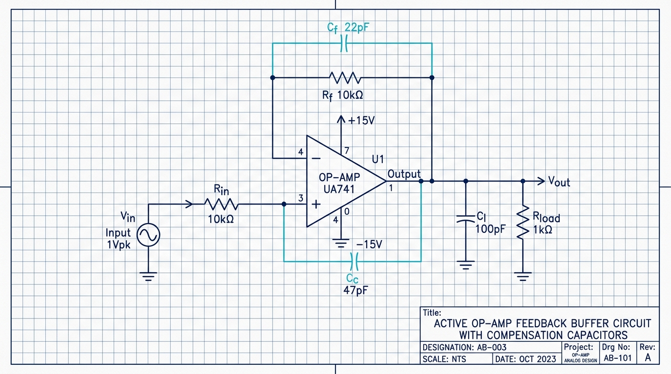
- Lead-Lag Compensation: Placing a feedback capacitor $C_f$ in parallel with the feedback resistor $R_f$ to introduce a zero, pulling the phase back up near the crossover frequency.
- In-loop RC Isolation: Inserting a small resistor in series with the op-amp output before the feedback node to decouple heavy capacitive loads.